10. Implementing HOG
Histogram of Oriented Gradients
HOG is also referred to as a type of feature descriptor, which is a simplified representation of an image that is made up of extracted features (that highlight important parts in an image) and that discards extraneous information. In this case the features represent the image gradient -- it's magnitude and directions, which describe the shapes and patterns of intensity that make up the image.
Implementing HOG
There are a number of steps to create a HOG feature vector, and we'll go through them here. It's also important to note that many image sets require pre-processing as a first step to ensure consistency in size and color, but we will gloss over that here to better focus on HOG.
For this example, we'll be looking at a small dataset of car images.
Note: The below code is to emphasize HOG steps and not for copy-and-paste usage.
1. Gradient Magnitude and Direction
First, HOG relies on calculation of the image gradient at each pixel; it's magnitude and direction. And we already know how to calculate these values: with Sobel filters! In the below code, I am using OpenCV's Sobel function instead of creating my own filter.
# Read in your image and convert to grayscale
image = cv2.imread('car1.jpg')
image = cv2.cvtColor(image, cv2.COLOR_BGR2RGB)
gray = cv2.cvtColor(image, cv2.COLOR_RGB2GRAY)

# Compute the gradients in the x and y directions
gx = cv2.Sobel(gray, cv2.CV_32F, 1, 0)
gy = cv2.Sobel(gray, cv2.CV_32F, 0, 1)

# Compute the magnitude and direction of the image gradient
mag, ang = cv2.cartToPolar(gx, gy)
2. Define the Cells and Bins
Next, we'll want to define how we divide this data into a histogram.
As in the video, I'll define 9 bins for 9 different ranges of gradient directions. And for the 64x64 image, this will break nicely into 8x8 cells for analysis.
# Creating bin ranges
n_bins = 9
bins = np.int32(n_bins*ang/(2*np.pi))
3. Calculate the Histogram for each Cell
With these values in mind, we know that we have 64 total 8x8 cells, and for each of these, we calculate a histogram of directions (9 bins) weighted with their magnitude. So, each cell will produce a feature vector containing 9 values. Sixty-four of those together (that form the complete 64x64 image) give us a complete image feature vector containing 576 values. This is almost the feature vector we use to train our data!
One more step that HOG does before creating the feature vector is to perform block normalization. A block is a larger area than a cell and checks different positions for the cell, determining how much they overlap.
So, the HOG features for all cells in each block are computed at each block position and the block shifts across and down through the image cell by cell.
So, the actual number of features in your final feature vector will be the total number of block positions multiplied by the number of cells per block, times the number of orientations, or in the case shown below: 7\times7\times2\times2\times9 = 1764.
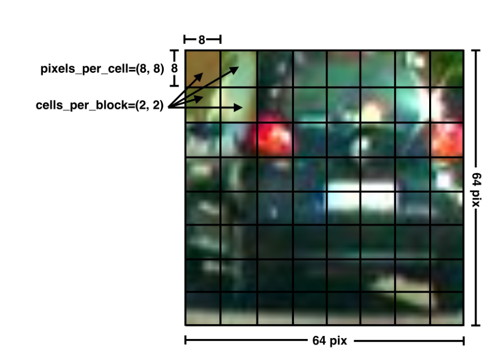
HOG cell breakdown for a car image
OpenCV HOG Descriptor
Now, that's a lot of steps to keep track of, and OpenCV has a function to help us perform the complete HOG algorithm with defined blocks and cells.
# Parameters you define for a HOG feature vector
win_size = (64, 64)
block_size = (16, 16)
block_stride = (5, 5)
cell_size = (8, 8)
n_bins = 9

# Create the HOG descriptor
hog = cv2.HOGDescriptor(win_size, block_size, block_stride, cell_size, n_bins)

# Using the descriptor, calculate the feature vector of an image
feature_vector = hog.compute(image)
The feature vector that this produces is what you can use to train a classifier!